Continual Learning, Compositionality, and Modularity - Part Ⅱ

Created by Yuwei Sun
All posts

Modular Neural Networks and Transfomers

Modular Neural Networks (MNNs) introduce sparsity in neuron connections between neural network layers. MNNs are divided into smaller, more manageable parts, they can be trained more efficiently and with fewer resources than a traditional, monolithic neural network.Usually, a larger model and more training samples contribute to the improvement of task performance, nevertheless, the computational cost also increases greatly with the increasing model parameters. MNNs permits the training of a large, sparse model without increasing the computational cost.

Previous work showed that MNNs could retain competitive/better performance compared with SOTA monolithic models, with better generalization to unseen data, notably, when pretrained with a large dataset and finetuned on the target dataset. MNNs learn independent experts to tackle different input samples/sample patches [1], increasing its interpretability. If a problem arises in a modular neural network, it is easier to identify the specific module that is causing the issue, especially in areas that necessitate explainability like healthcare.

Definition of Modular Neural Networks

Let $x\in\mathbb{R}^P$ be a sample and $y \in \{1,2,...,C\} = Y$ be a label, where $C$ is the total number of categories. $D$ consists of a collection of $N$ samples as $D=\{(x_i, y_i)\}_{i=1}^N$. In a modular neural network layer, each sample $x$ is processed sparsely by $K$ out of $E$ available experts $\{\mbox{MLP}_e\}_{e=1}^E$. These experts usually share the same architecture (e.g. a multilayer perceptron) but different model parameters. To choose which $K$, a router $g(\cdot)$ (a neural network) predicts the gating weights $W_g$ per sample $x$. $g(x)=\mbox{softmax}(W_g)\in\mathbb{R}^E$ with learned $(W_gx)\in\mathbb{R}^{P\times E}$. The outputs of the $K$ activated experts are linearly combined according to the gating weights. $\mbox{MoE}(x) = \sum_{e=1}^K g(x)_e\cdot \mbox{MLP}_e(x)$.

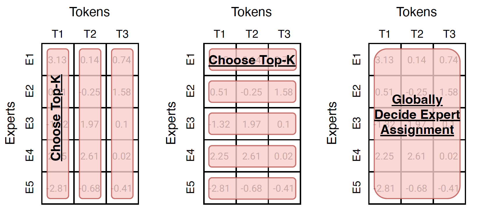
One way to understand many routing algorithms is to analyze the matrix of routing scores (weights) as shown in Figure 1.

To introduce sparsity into a monolithic model like Vision Transformer (ViT) [7], we replace several fully-connected (FC) layers of ViT with the modular layer comprised of experts. For each modular layer, a different routing function is applied.

Related Work

In Computer Vision, almost all performant networks are “dense”, that is, every input is processed by every parameter. Conditional computation [8] aims to increase model capacity while keeping the training and inference cost roughly constant by applying only a subset of parameters to each example. Mixture-of- experts (MoEs) model is a specific instantiation

Scaling Vision with Sparse Mixture of Experts [9]

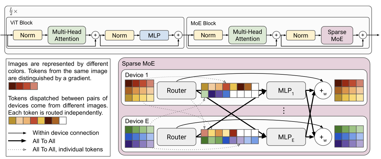
This work presented a Vision Mixture of Experts (V-MoE) (Figure 2), a sparse version of the Vision Transformer (ViT)[7], that is scalable and competitive with the largest dense network ViT, reducing half of the compute at inference time.

The main contributions of the V-MoE are as follows: 1. The V-MoE replaces a subset of the dense feedforward layers in ViT with sparse MoE layers, where each image patch is “routed” to a subset of “experts” (MLPs). 2. Batch Prioritized Routing, a routing algorithm that repurposes model sparsity to skip the computation of some patches, reducing compute on uninformative image regions.

Model Architecture of MoEs

The model of an expert $e_i$ comprises two layers and a GeLU non-linearity$\sigma_{gelu}(\cdot)$. $e_i(x) = W_2\sigma_{gelu}(W_1x)$. The experts have the same architecture but with different weights $\theta_i = (W_1^i,W_2^i)$.

Routing

For each MoE layer, a rounting function $g(x)=\mbox{TOP}_k(\mbox{softmax}(Wx+\epsilon))$ is employed, where $\mbox{TOP}_k$ is an operation that sets all elements of the vector to zero except the elements with the largest $k$ values, and $\epsilon$ denotes the noise sampled independently $\epsilon \sim \mathcal{N}(0,\frac{1}{E^2})$ where $E$ is the expert number. The noise typically alters routing decisions ~15\% of the time in earlier layers, and ∼2–3\% in deeper layers.

Allocation Load Balancer

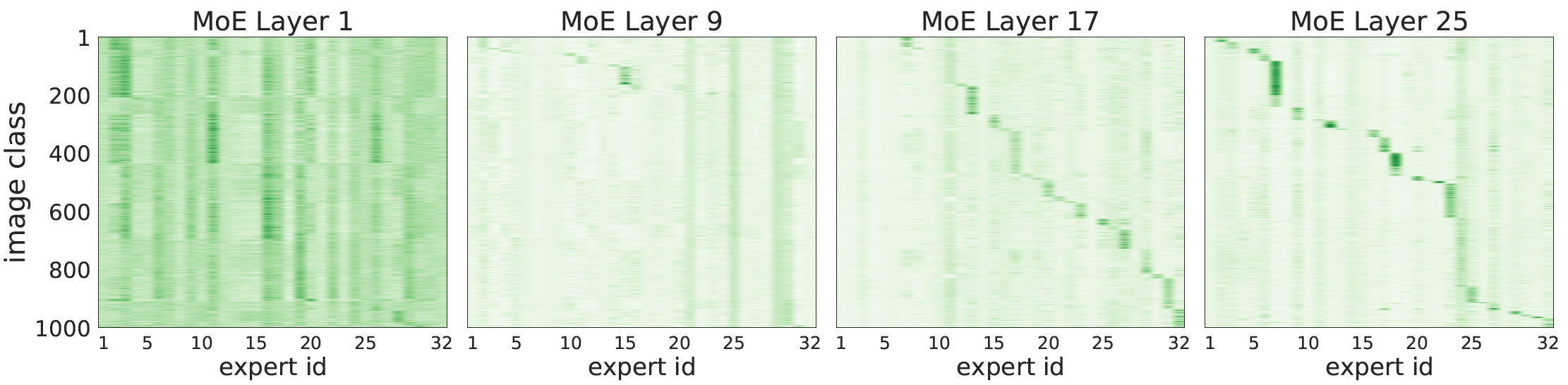
During training, sparse models may favor only a small set of experts. Setting the expert's buffer capacity permits that if the router assigns more than $B_e$ tokens to a given expert, only $B_e$ of them are processed. The remaining tokens are preserved by residual connections to the next layer. In contrast, if an expert is assigned fewer than $B_e$ tokens, the rest of its buffer is zero-padded. The authors used by default $\mbox{TOP}_2$ and a total number of experts $E = 32$ for each modular layer. Figure 3 shows the routing decisions correlated with image classes. In earlier MoE layers we do not observe expert sparsity. That's because experts may instead focus on aspects common to all classes (background, basic shapes, colors).

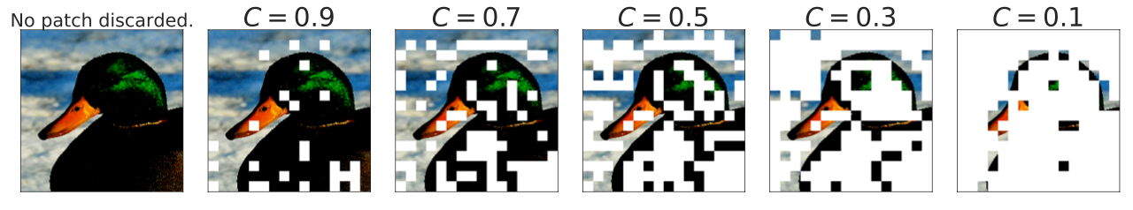
Batch Prioritized Routing

In Vanilla routing, for $i < j$, every TOP-$i$ assignment has priority (be first processed) over any TOP-$j$ assignment. The router first tries to dispatch all $i$th expert choices before assigning any $j$th choice. As a result, priority is given to tokens depending on the rank of their corresponding row. While images in a batch are randomly ordered, tokens within an image follow a pre-defined fixed order. To favour the “most important” tokens, a priority score $s(x)$ on each token $x$ is computed and sorted before proceeding with the allocation. This is based on their maximum routing weight, $s(x)_t = \mbox{max}_i g(x)_{t,i}$ or the sum of TOP-$k$ weights, $s(x)_t = \sum_i g(x)_{t,i}$ (Figure 4).

Sparse MoEs meet Efficient Ensembles [1]

They proposed the efficient ensemble of experts ($E^3$). Building upon V-MoE [9], this work studies the interplay of two popular classes of such models: ensembles of neural networks and sparse mixture of experts (sparse MoEs). Ensemble methods combine several different models to improve generalization and uncertainty estimation. We assume a set of $M$ model parameters $\Theta=\{\theta_m\}_{m=1}^M$. Prediction proceeds by computing $\frac{1}{M}\sum_{\theta\in\Theta}f(x;\theta)$, i.e., the average probability vector over the $M$ models.

Disjoint subsets of experts

$E^3$ partitions the set of $E$ experts into $M$ subsets of $E/M$ experts. The ensemble members have separate parameters for independent predictions, while efficiently sharing parameters among all non-expert layers. Instead of having a single routing function, $E^3$ applies separate routing functions $\mbox{gate}_K(W_m\cdot)$ to each subset $\mathcal{E}_m$.

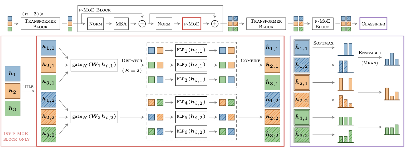
Tiled representation

To jointly handle the predictions of the $M$ ensemble members, we tile the inputs by a factor $M$. A given image patch has $M$ different representations that, when entering an MoE layer, are each routed to their respective expert subsets $\mathcal{E}_m$ (Figure 5). Consider some tiled inputs $H \in \mathbb{R}^{B\times M\times D}$ where $B$ refers to total image patches number and $h_{i,m} \in \mathbb{R}^D$ is the representation of the $i$-th input for the $m$-th member. The routing is as follows

$$\mbox{p-MoE}(h_{i,m})=\sum_{e\in\mathcal{E}_m}g_e(h_{i,m})\cdot \mbox{MLP}_e(h_{i,m}),$$

where $\{g_e(h_{i,m})\}_{e\in\mathcal{E}_m}=\mbox{gate}_K(W_m h_{i,m})$ and $W_m\in\mathbb{R}^{(E/M)\times D}$.

Taming Sparsely Activated Transformer with Stochastic Experts [10]

Sparsely activated models (SAMs), such as Mixture-of-Experts (MoE), are reported to be parameter inefficient where larger models do not always lead to better performance. This work showed that the commonly-used routing methods based on gating mechanisms do not work better than randomly routing inputs to experts. They proposed a new expert-based model, THOR (Transformer witH StOchastic ExpeRts), where experts are randomly activated (with no need of any gating mechanism) for each input during training and inference. THOR models are trained by minimizing both the cross-entropy loss and a consistency regularization term, such that experts can learn not only from training data but also from other experts as teachers.

The stochastic expert routing tackles the problem of load imbalance (Figure 6). Existing works adopt various ad-hoc heuristics to mitigate this issue, e.g., adding Gaussian noise (noisy gating [11]), limiting the maximum number of inputs that can be routed to an expert (expert capacity [4]), imposing a load balancing loss [4][12], and using linear assignment [7].

In an iteration, a pair of experts are activated in THOR. Two prediction probabilities produced by the two selections are $p_1 = f(x; \{E_i^l\}_{l=1}^L)$ and $p_2 = f(x; \{E_j^l\}_{l=1}^L)$. Then, the training objective of THOR with respect to training samples $(x,y)$ in the dataset $D$ is

$$\mbox{min}\sum_{(x,y)\in D}\ell(x,y)=\mbox{CE}(p_1;y)+\mbox{CE}(p_2;y)+\alpha\mbox{CR}(p_1;p_2),$$

where $\mbox{CR}(p_1;p_2)=\frac{1}{2}(\mbox{KL}(p_1||p_2)+\mbox{KL}(p_2||p_1))$. CE is the cross-entropy loss, CR is the consistency regularizer, and $\alpha$ controls the strength of the regularization.