Continual Learning, Compositionality, and Modularity - Part Ⅰ

Created by Yuwei Sun
All posts


This blog is the start of a series of blogs on continual learning.

Continual Learning

Disclaimer: the introduction part of this blog was written and modified with the help of ChatGPT.

Continual learning, also known as lifelong learning or incremental learning, refers to the ability of an artificial intelligence (AI) system to learn and adapt to new information and experiences over time, without forgetting previous knowledge. This is in contrast to traditional machine learning approaches, which typically involve training a model on a fixed dataset and then deploying it, with no further learning taking place. Continual learning is an active area of research in AI, with significant progress being made in recent years. However, there is still much work to be done to fully overcome the challenges of catastrophic forgetting and data efficiency, and to achieve truly lifelong learning in AI systems.

Several challenges must be overcome to achieve true continual learning in AI systems. One of the main challenges is the problem of catastrophic forgetting, which refers to the tendency of neural networks to forget previously learned knowledge when presented with new information. This can be a major problem in real-world applications, as it limits the ability of the system to learn and adapt over time.

To address this problem, researchers have proposed several approaches, including the use of modular networks, which allow different parts of the network to learn and adapt independently, and the use of memory-based methods, which store previously learned knowledge in a memory buffer and use it to make predictions on new data. In this part of the Continual Learning blog, we will first look into modular neural networks.

Another challenge in continual learning is the problem of data efficiency, which refers to the ability of the system to learn from a limited amount of data. In many real-world applications, it is not possible to obtain large amounts of labeled data for every new task or concept that the system needs to learn. To address this problem, researchers have proposed several methods, including transfer learning and meta-learning, which allow the system to transfer knowledge from previously learned tasks to new ones.

Compositionnality

Compositionality is the ability to understand and generate complex concepts or behaviors by combining simpler, more basic concepts or behaviors. Compositionality is often associated with the idea of building intelligent systems using modular components or "building blocks" that can be combined in different ways to perform a wide range of tasks or functions.

One of the key benefits of compositionality is that it allows a system to learn and adapt more efficiently, as it can build upon its existing knowledge and skills rather than starting from scratch each time it encounters a new task or concept. This can be particularly useful in the context of continual learning, where a system must be able to learn and adapt to new information and experiences over time, without forgetting previous knowledge. There are several approaches that have been proposed for achieving compositionality, including the use of modular networks and the use of meta-learning.

Modularity

Modularity refers to the idea of dividing a system into distinct, independent modules or components that can perform specific tasks or functions. Modularity can be useful in a number of ways. For example, it can make a system easier to design, build, and maintain, as each module can be developed and tested independently before being integrated into the overall system. Modularity can also make a system more flexible and adaptable, as different modules can be swapped in or out as needed to perform different tasks or functions.

In the context of neural networks, modularity allows multiple independent sub-networks or modules to form a neural network, each of which is responsible for learning a specific task or function. This can be useful for overcoming the problem of catastrophic forgetting in continual learning, i.e., the tendency of neural networks to forget previously learned knowledge when presented with new information. By dividing the network into modular components, it is possible to allow different parts of the network to learn and adapt independently, without disrupting the knowledge that has been learned by other parts of the network. In the next part, we review several of the most recent work on modular computation in neural networks.

Related Work

Routing Networks and the Challenges of Modular and Compositional Computation [1]

The authors identified and analyzed the underlying causes of several issues in Modular and Compositional Computation. As an example, this work studied the routing network (Figure 1).

Notably, they studied the “transfer-interference trade-off” problem for choosing which parameters in the model are shared across different input samples or distributions. When there is a large amount of sharing of model parameters during training we may see better performance as a consequence of the transfer since each parameter is trained on more data. But it may also lead to worse performance if the training on different samples produces updates that cancel each other out or cause interference. Compositional architectures can offer an interesting balance between the two, as different modules may be active for different samples.

Outrageously Large Neural Networks: The Sparsely-Gated Mixture-of-Experts Layer [2]

This work introduced a Sparsely-Gated Mixture-of-Experts layer (MoE), consisting of up to thousands of feed-forward sub-networks. A trainable gating network determines a sparse combination of these experts to use for each example, which scales up neural network models to handle larger datasets and more complex tasks (Figure 2).

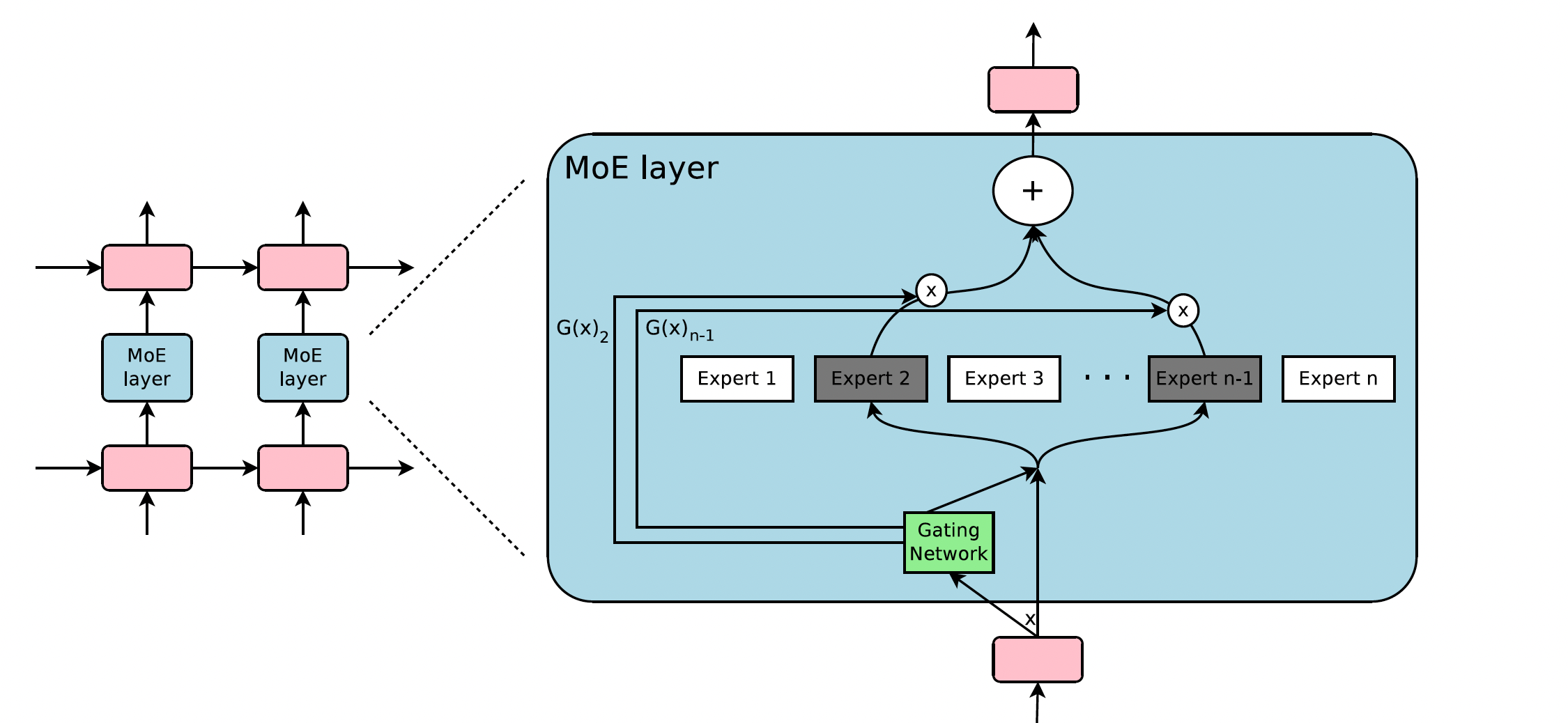
The authors propose a new variant of the MoE layer called the sparsely-gated MoE layer, which is designed to improve the scalability and efficiency of MoE layers. The sparsely-gated MoE layer uses a sparse gating function to control the flow of information within the network, allowing it to selectively activate a subset of expert networks in the MoE layer and effectively prune the number of computations required.

Learning to Prompt for Continual Learning [3]

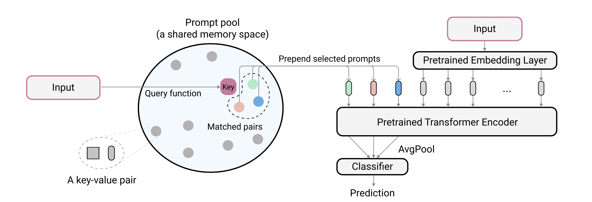
The authors proposed the learning to prompt (L2P), a novel continual learning framework based on prompts for continual learning through learning a prompt pool memory space (Figure 3). Task-specific knowledge is stored inside a prompt pool, thus a rehearsal buffer is no longer mandatory to mitigate forgetting. L2P automatically selects and updates prompt from the pool in an instance-wise fashion, thus task identity is not required at test time.

At training time, first, L2P selects a subset of prompts from a key-value paired prompt pool based on an instance-wise query mechanism. Then, L2P prepends the selected prompts to the input tokens. Finally, L2P feeds the extended tokens to the model and optimizes the prompt pool through the loss defined below. The objective is to learn to select and update prompts to instruct the prediction of the pre-trained backbone model.

$$K_x = \underset{\{s_i\}_{i=1}^N \subseteq[1,M]}{\mbox{arg min}} \sum_{i=1}^{N} \gamma(q(x),k_{s_i}), $$

where $K_x$ represents the subset of top-$N$ keys selected specifically for $x$ from $K$ and $q$ is a function to score the match between the query and prompt key (cosine distance here).

Then the loss is defined by:

$$\mathcal{L}(g_{\phi}(f_r^{avg}(x_p)),y)+\lambda\sum_{K_x}\gamma(q(x),k_{s_i}),$$

where the first term is the softmax cross-entropy loss, and the second term is a surrogate loss to pull selected keys closer to corresponding query features. $\lambda$ is a scalar to weigh the loss.

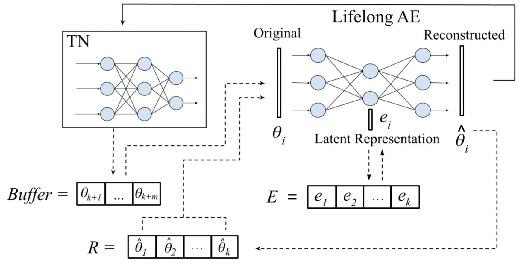
Self-Net: Lifelong Learning via Continual Self-Modeling [4]

This work proposed Self-Net (Figure 4) that uses an autoencoder to learn a set of low-dimensional representations of the weights learned for different tasks. These low-dimensional vectors can then be used to generate high-fidelity recollections of the original weights. Self-Net can incorporate new tasks over time with little retraining, minimal loss in performance for older tasks, and without storing prior training data.

Given new tasks $\{t_{k+1}, \dots, t_{k+m}\}$, where $k$ is the number of tasks previously encountered, Self-Net first trains $m$ task-networks independently to learn $\{\theta_{k+1}, \dots, \theta_{k+m}\}$ optimal parameters for these tasks. These networks are temporarily stored in the Buffer. When the Buffer fills up, Self-Net incorporates the new networks into long-term representation by retraining an autoencoder on both its approximations of previously learned networks and the new batch of networks. When an old network is needed (e.g., when a task is revisited), the weights are reconstructed and loaded onto the corresponding TN. The reconstructed network closely approximates the performance of the original.

Multimodal Contrastive Learning with LIMoE: the Language-Image Mixture of Experts [5]

The primary motivation for using a mixture of experts (MoEs) is to scale model parameters while keeping compute costs under control. These models however have other benefits; for example, the sparsity protects against catastrophic forgetting in continual learning and can improve performance for multi-task learning by offering a convenient inductive bias.

Transformer backbone

The authors employed a single Transformer-based architecture (Figure 5) for both image and text modalities. The preprocessed pairing image and text representations $z_{i_k}$ and $z_{t_k}$ are linearly projected using per-modality weight matrices $W$. $\{(W_{\mbox{image}}z_{i_k}, W_{\mbox{text}}z_{t_k})\}_{k=1}^n$.

Multimodal contrastive learning

Given $n$ pairs of images and text captions $\{(i_j,t_j)\}_{j=1}^n$, the model learns representations $Z_n=\{(z_{i_j},z_{t_j})\}_{j=1}^n$ such that those corresponding to paired inputs are closer in feature space than those of unpaired inputs, based on a contrastive learning objective.

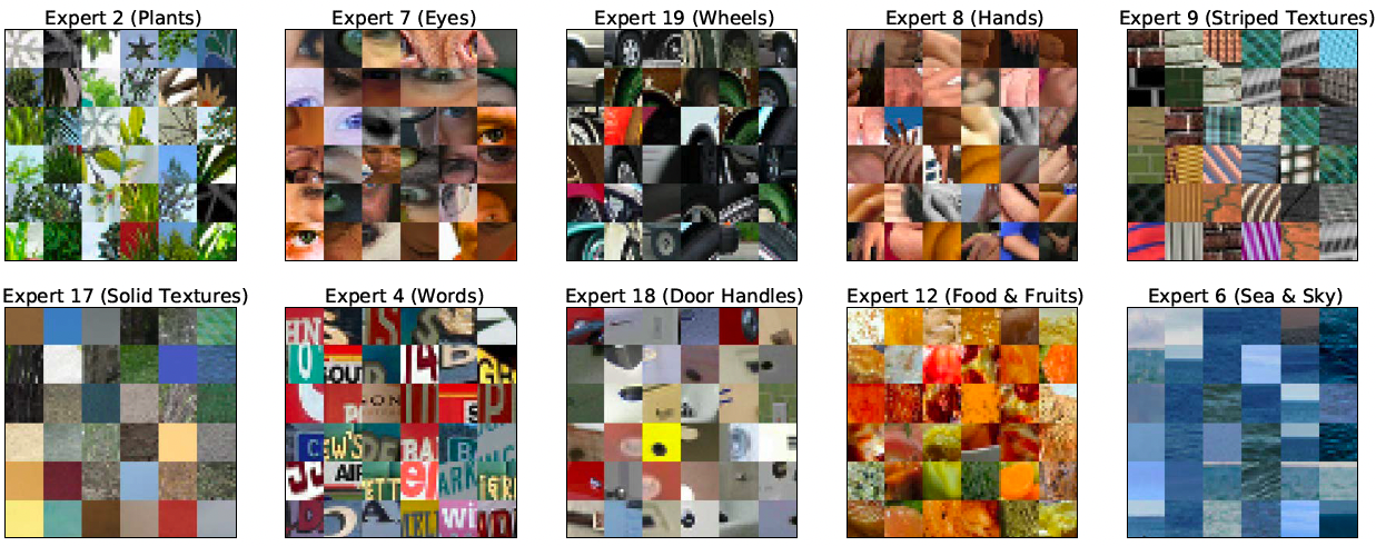
Sparse MoE backbone

LIMoE contains multiple MoE layers. In those layers, each token $x\in\mathbb{R}^D$ is processed sparsely by $K$ out of $E$ available experts (Figure 6). To choose which $K$, a lightweight router predicts the gating weights per token. $g(x)=\mbox{softmax}(W_gx)\in\mathbb{R}^E$ with learned $(W_gx)\in\mathbb{R}^{D\times E}$. The outputs of the $K$ activated experts are linearly combined according to the gating weights. $MoE(x) = \sum_{e=1}^K g(x)_e\cdot \mbox{MLP}_e(x)$.

Note that, for computational efficiency and implementation constraints, experts have a fixed buffer capacity. The number of tokens each expert can process is fixed in advance and typically assumes that tokens are roughly balanced across experts. If capacity is exceeded, some tokens are “dropped”; they are not processed by the expert, and the expert output is all zeros for those tokens. The rate at which tokens are successfully processed (that is, not dropped) is referred to as the “success rate”. It is an important indicator of healthy and balanced routing and is often indicative of training stability.

To tackle challenges in multimodal MoEs, i.e., module collapse and modality misbalance. This work further introduced two new losses the local entropy loss and the global entropy loss.

$$\Omega_{\mbox{local}}(G_m):=\frac{1}{n_m}\sum_{i=1}^{n_m}\mathcal{H}(p_m(\mbox{experts}|x_i)),$$ $$\Omega_{\mbox{global}}(G_m):=-\mathcal{H}(\tilde{p_m}(\mbox{experts})),$$

where $\tilde{p_m}(\mbox{experts}) = \frac{1}{n_m}\sum_{i=1}^{n_m}p_m(\mbox{experts}|x_i)$ is the expert probability distribution averaged over the tokens and $\mathcal{H}(p)=-\sum_{e=1}^E p_e\mbox{log}(p_e)$ denotes the entropy. $\Omega_{\mbox{local}}$ applies the entropy locally for each token while $\Omega_{\mbox{global}}$ applies the entropy globally after having marginalized out the tokens.