Neural Network Approaches to the Binding Problem

Created by Yuwei Sun
All posts

Inspirations from Neuroscience

Neurons in all animals form a net in which every neuron has a single axon that branches and contacts the dendrites of other neurons at synapses, where the simultaneous firing pattern of large populations of cells carries the information [1]. There is no rigid layer structure in the cortex and neural nets often work better when there are layer-skipping links. This suggests that a new kind of transformer is needed for this, something with queries and values in the original net and keys in the new higher layers. Neural nets need to have something like memory at higher levels and feedback at lower levels, to be more modular and to have structures specific for both feedforward and feedback data exchange. Memory traces (old events) are merged as much as possible with the new sensory input and new situation.

Binding Problem [2]

Contemporary neural networks still fall short of human-level generalization, showing an inability to dynamically and flexibly bind information that is distributed throughout the network. Connectionism takes a brain-inspired, approach that stands in contrast to symbolic AI and its focus on the conscious mind. Evidence indicates that neural networks learn mostly about surface statistics in place of the underlying concepts.

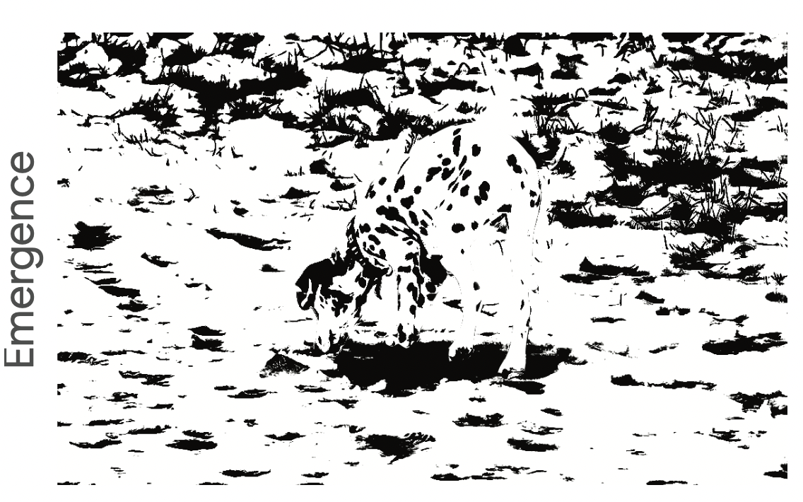
Attractor dynamics is an approach for addressing representational dynamics in binding. Early work includes Hopfield networks, Boltzmann machines, and associative memory. Attractor states were also found to occur in RNNs. A dynamical segregation process has multiple stable equilibria that each correspond to a particular decomposition of a given scene. The concept of Emergence refers to the sudden transition process from the perception as an unstructured collection of patches on a background to a meaningful scene (Figure 1), where the perception of the whole arises at once, and not through the hierarchically assembling of parts.

Memory

Neurons that fire together wire together [3]. Associative memory, also called content-addressable memory, organizes information according to its “meaning” or its relationship to other stored information. The overlap of content among distributed representations forms the associate network of stored information. In neuroscience, such memory is stored in the hippocampus, where high-level features of information from the cortex are encoded. Working memory in neurophysiology means a capacity for short-term storage of information and its rule-based manipulation [4]. In machine learning, recurrent neural networks (RNNs) have larger working memory and computational capacity because their state evolves based on both input and current state. Other types of external memory for neural networks have been proposed, including continuous stacks, grid and tape storage, memory networks, and attention-based neural networks. These models have been successfully applied to various tasks such as machine translation, speech recognition, and image caption generation.

Experience Richness and Ineffability in Working Memory [5]

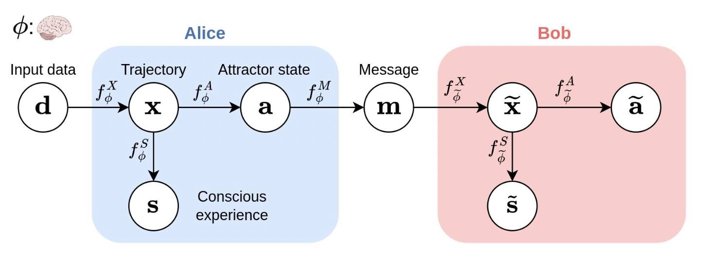
The richness of conscious experience corresponds to the amount of information in a conscious state and ineffability corresponds to the amount of information lost at different stages of processing (Figure 2). To quantitatively measure the richness of conscious experience (a trajectory $X$ of states), its entropy $H(X)$ is measured using the Information Theory. Given a function that processes the input states $X$ and produces an output variable $Y$, the ineffability incurred by the output is measurable by conditional entropy $H(X|Y) = H(X)−I(X;Y)$, where $I(X;Y)$ is the mutual information between $X$ and $Y$.

Discretization

Composing elements and their relations together into more complex elements, and vice versa, to decompose complex elements into simpler elements, is regarded as crucial to human intelligence [6]. Language and other symbolic representations are, by nature, compositional. The syntactical structure of natural language allows for the replacement of words in sentences so that they acquire another meaning. One potential underlying reason for discretization is the more excellent information-theoretic signaling reliability and efficiency in communicating symbols versus continuous signals [7]. Historically, many neural networks also featured discrete-valued nodes, like (restricted) Boltzmann machines or Hopfield networks [8]. Nevertheless, the problem is making discrete, non-differentiable processing amenable to gradient-based learning. Combining continuous representations of neural networks and discrete representations of symbols and elements will be essential to build systems that exhibit a general form of intelligence [9]. For example, using continuous representations as attributes in discretely structured graph representations gives a form of hybrid representation and adds structure to neural network processing.

Inductive Biases in Knowledge Representation [10]

There are two types of knowledge representation, that is implicit knowledge and explicit knowledge. Implicit knowledge (system 1) is intuitive and difficult to verbalize; explicit knowledge (system 2) allows humans to share part of their thinking process through natural language. To represent explicit knowledge, declarative knowledge such as Monte-Carlo Markov chains (facts, hypotheses, and causal dependencies) and inference machinery to reason with these pieces of knowledge. In addition, when a new rule is introduced, move back some of system 1 processing to system 2 to avoid inconsistencies. The no-free-lunch theorem for machine learning says that some set of inductive biases is necessary to obtain generalization, and that there is no completely general-purpose learning algorithm. Inductive biases encourage the learning algorithm to prioritize solutions with certain properties.

Related Work

Classical Hopfield Network [11]

Classical Hopfield network consists of neurons connected by symmetric weights. Then based on stored patterns, the model updates its weights to arrive at a stable state in its dynamic systems. These patterns settle down at various attractors of the dynamic systems, each of which has a basin of attraction. When an incoming state is inside an attractor’s attraction region, the Hopfield network will evolve the dynamics of the system to the closest stored pattern for the given initial state, by using a Lyapunov function in the form of free energy. Then for each step of evolving, the object of the model is to decrease the overall energy of the system since a state with lower energy is more stable. Therefore, an intact pattern can be recalled using parts of the pattern when the initial state defined by the part is located in the attractor’s region of attraction. The process of a pattern moving towards a stored attractor pattern is similar to the process of discretization. And this process allows a Hopfield network to quickly recall patterns (attractors) with a few samples.

In classical Hopfield Networks, the simplest associative memory is realized by a sum of outer products of the $N$ patterns $\{x_i\}^N_{i=1},\,x_i∈\{−1,1\}^d$ that we want to store based on the Hebbian learning rule, where $d$ is the length of the patterns. $W = \sum_{i=1}^{N}x_i x_i^T$, where $W$ is the weight matrix and $x_i$ is an initial state pattern. Furthermore, for the recall of a stored pattern, a total of two steps’ updates with an asynchronous method are conducted, where the update of each node’s state is conducted in succession with a random start node. And the dynamic systems of the Hopfield network continue moving to the state of lower energy during the updates, until it converges to a stable state with the minimum potential energy. By this approach, an input test pattern with partially shared features with one of the stored patterns can be reconstructed to the intact stored pattern. Nevertheless, the main issue of the traditional Hopfield network is that it is non-differentiable and not applicable to gradient-based learning. We now look into a modern version of the Hopfield network.

Modern Hopfield network

The discrete modern Hopfield Networks were proposed by Krotov and Hopfield [12], and subsequently further developed by Demircigil et al. [13] to increase the storage capacity of the network. Ramsauer et al. [14] proposed a new energy function as follows for continuous-valued patterns and states for processing continued-value patterns.

$$E = -\mbox{lse}(\beta, x_i^T \xi) +\frac{1}{2} \xi^T \xi + \beta^{-1} \ln N + \frac{1}{2}M^2,$$

which is constructed from $N$ continuous stored patterns by the matrix $X=(x_1,\dots,x_N)$, where $M$ is the largest norm of all stored patterns. They are continuous and differentiable with respect to their parameters. Moreover, they typically retrieve patterns with one update, which is conform to deep learning layers that are activated only once. For these two reasons, modern Hopfield networks can serve as specialized layers in deep networks to equip them with memories, called the layer Hopfield [14]. The update rule for a state pattern $\xi$ is given by:

$$\xi_{new} = X\,\mbox{softmax}(\beta X^T \xi)$$

The layer Hopfield propagates sets of vectors via state (query) patterns $R$ and stored (key) patterns $Y$. Several major design decisions that affect the cost and quality of the discretization process includes:

Update steps

Multiple updates control how precise fixed points are found without additional parameters needed. We use by default three updates in one Hopfield head with total eight parallel association heads. The update can be iteratively applied to the initial state of every Hopfield layer head. After the last update, the new states are projected to the result patterns. Therefore, the Hopfield layer allows multiple update steps in the forward pass without changing the number of parameters. The number of update steps can be given for every Hopfield head individually.

Inverse temperature $\beta$

The Hopfield network's iterative process converges to a fixed point that is close to one of the stored patterns. However, if some of the stored patterns are similar to each other, a metastable state, which is near these similar patterns, can appear. The iterates that start close to this metastable state or at one of the similar patterns will converge to this metastable state. Such learning dynamics of the network can be controlled by adjusting the value of the inverse temperature, $\beta$ ($\beta = 0.25$ by default). A high value of $\beta$ makes it less likely for metastable states to appear, while a low value of $\beta$ increases the likelihood of the formation of metastable states.

Dimension of the associative space $d_k$

The storage capacity of the modern Hopfield network grows exponentially with the dimension of the associative space. However higher dimension of the associative space also means less averaging and smaller metastable states. The dimension of the associative space trades off storage capacity against the size of metastable states, e.g. over how many pattern is averaged. $d_k$ should be chosen with respect to the number $N$ of patterns one wants to store and the desired size of metastable states, which is the number of patterns one wants to average over. For example, if the input consists of many low dimensional input patterns, it makes sense to project the patterns into a higher dimensional space to allow a proper fixed point dynamics. We use $d_k = 8$ by default.

Comparison to Transformers

The Hopfield layer enables multiple updates (iterating the attention) with adjustable $\beta$ in place of Transformers' $1/\mbox{sqrt}(d_k)$ scaling factor and flexible integration in arbitrary deep network architectures. Transformers perform the attention in a single step, though iterating the Hopfield attention doesn't seem to be beneficial.

Neural Turing Machines [15]

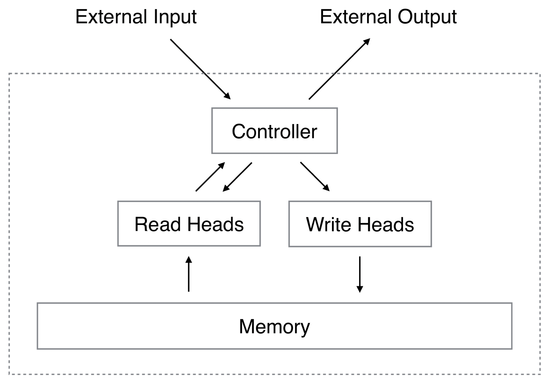
Neural Turing Machines (NTM) extend the capabilities of neural networks by coupling them to external memory resources, which they can interact with by attentional processes. NTM contains two basic components: a neural network controller (either a feed-forward network or an LSTM network) and a memory bank (Figure 3). Every component of the architecture is differentiable, making it straightforward to train with gradient descent.

Memory Bank

The memory bank is realized using specialised outputs emitted by the two heads, i.e., the read and write head. These outputs define a normalised weighting over the rows in the memory matrix, representing the degree to which the head reads or writes at each location.

Read head

Let $M_t$ be the contents of the $N \times M$ memory matrix at time $t$, where $N$ is the number of memory locations, and $M$ is the vector size at each location. Let $w_t$ be a vector of weightings over the $N$ locations emitted by a read head at time $t$.

$$ \sum_i w_t(i) = 1,\,0 \leq w_t(i) \leq 1, \forall i.$$

The read vector $r_t$ with a length $M$ returned by the head is defined by:

$$r_t = \sum_i w_t(i)M_t(i).$$

Write head

Each write head consists of an erase followed by an add. Given a weighting $w_t$ of the write head, an erase vector $e_t$ whose $M$ elements all lie in the range (0,1), updates the memory vectors as follows:

$$\tilde{M}_t(i) = M_{t−1}(i)[1 − w_t(i)e_t].$$

The elements of a memory location are reset to zero only if both the weighting at the location and the erase element are one; if either the weighting or the erase is zero, the memory is left unchanged.

Each write head has an $add\,vector\,a_t$, which is added to the memory after the erase step:

$$M_t(i) = \tilde{M}_t(i)+ w_t(i)a_t.$$

Addressing

Content-based addressing: focuses attention on locations based on the similarity between their current values and values emitted by the controller. This is related to the content-addressing of Hopfield networks.

Each head produces a length $M key vector k_t$ that is compared to each vector $M_t(i)$ by a similarity measure. Then, a normalised weighting $w_t^c$ based on the similarity and a positive key strength $\beta_t$ is computed:

$$w_t^c(i) = \frac{\mbox{exp}(\beta_t K[k_t, M_t(i)])}{\sum_j \mbox{exp}(\beta_t K[k_t, M_t(j)])},$$ $$K[u,v] = \frac{u\cdot v}{||u||\cdot ||v||},$$

where $K[u,v]$ is the cosine similarity.

Location-based addressing: is designed to facilitate both simple iteration across the locations of the memory and random-access jumps by implementing a rotational shift of a weighting.

$$w_t^g = g_t w_t^c + (1 − g_t)w_{t−1},$$

where $g_t$ is a coefficient.

$s_t$ defines a normalised distribution over the allowed integer shifts. For example, if shifts between -1 and 1 are allowed, $s_t$ has three elements corresponding to the degree to which shifts of -1, 0 and 1 are performed. The rotation applied to $w_t^g$ by $s_t$ can be expressed in the following:

$$\tilde{W}_t(i) = \sum_{j=0}^{N-1}w_t^g(j)s_t(i-j).$$

Furthermore, a scalar $\gamma_t \geq 1$ is used to sharpen the final weighting as follows:

$$w_t(i)=\frac{\tilde{W}_t(i)^{\gamma_t}}{\sum_j \tilde{W}_t(j)^{\gamma_t}}.$$

Dynamic Neural Turing Machine [16]

Dynamic neural Turing machine (D-NTM) extends NTM by introducing a learnable addressing scheme which allows the NTM to be capable of performing highly nonlinear location-based addressing. Similar to NTM, D-NTM consists of a controller (either a gated recurrent unit (GRU) network or a feed-forward network) and a memory bank.

Different from NTM, for each cell in the memory bank $M \in \mathbb{R}^{N\times(d_c +d_a)}$, it has two parts, i.e., a learnable address matrix $A$ (read, write and erase) and a content matrix $C$ s.t. $C_0 = 0$. The address part $a_i$ is considered a model parameter that is updated during training. During inference, the address part remains constant. On the other hand, the content part $c_i$ is modified by the controller both during training and inference. The learnable address allows the model to learn sophisticated location-based addressing strategies.

For writing and erasing, the memory matrix $C$ is updated by:

$$C^t[j]=(1-e^tu_j^t)\odot C^{t-1}[j]+u_j^t \bar{c}^t,$$

where $e^t,u_j^t,\bar{c}^t$ are the erase, write, and candidate memory content vectors, respectively. The candidate memory content vector is computed based on the current hidden state and the scaled input of the controller (GRU).

No Operation memory cell

In addition, an additional No Operation (NOP) action is designated to a memory cell, where reading or writing from this memory cell is ignored. That's because it might be beneficial for the controller not to access the memory once in a while.

Discrete addressing

An address vector (either read, write or erase) at time $t$ is converted to a one-hot vector for discretization. By further using a curriculum learning strategy, at the beginning of the training, the model learns to use the memory mainly with the continuous attention. As learning progresses, the model will rely more on the discrete attention.

Discrete-Valued Neural Communication (DVNC) [17]

Discrete-Valued Neural Communication (DVNC) learns a common codebook that is shared by all components for representation discretization and inter-component communication. DVNC achieves a much lower noise-sensitivity bound while allowing high expressiveness through the use of multiple discretization heads. For more detail on DVNC, please refer to a previous blog Global Workspace Theory and System 2 AI.

Dense Associative Memory for Pattern Recognition [18]

Dense associative memory is a recurrent network in which every neuron can be updated multiple times. In the case of associative memory the network stores a set of memory vectors. In a typical query the network is presented with an incomplete pattern resembling, but not identical to, one of the stored memories and the task is to recover the full memory, by properly designing the energy function (or Hamiltonian) for these models with higher order interactions. To mimic biology, the output should be small or zero if the input is below the threshold, but it is much less clear what the behavior of the activation function should be for inputs exceeding the threshold.The capacity of this model, which is the maximal number of memories that the network can store and reliably retrieve, is 0.14$N$. $N$ is the number of binary neurons in the associtive memory systems. The reason why the model (1) gets confused when many memories are stored is that several memories produce contributions to the energy which are of the same order. In other words the energy decreases too slowly as the pattern approaches a memory in the configuration space. To tackle this problem, a new energy function was introduced:

$$E = -\sum^K_\mu F(\xi^{\mu}_i\sigma_i) $$

When $n = 2$ the network reduces to the standard model of associative memory. If $n > 2$, each term becomes sharper, thus more memories can be packed into the same configuration space. The system updates a unit, given the states of the rest of the network, in such a way that the energy of the entire configuration decreases. One step update of the classification neurons is sufficient to bring this initial state to the nearest local minimum, thus completing the memory recovery, if the stored patterns are stable and have basins of attraction around them of at least the size of one neuron flip. The upper limit on the number of patterns that the network can store is as follows:

$$K^{\mbox{max}}=\alpha_n N^{n-1},$$

where $\alpha_n$ is a numerical constant. The case $n = 2$ corresponds to the standard model of associative memory and gives $K = 0.14N$.

The visible neurons, one for each pixel, are combined together with 10 classification neurons in one vector that defines the state of the network. The visible part of this vector is treated as an “incomplete” pattern and the associative memory is allowed to calculate a completion of that pattern, which is the label of the image. For higher powers $n$, the speed-up of convergence is larger, especially for a large dataset. An input is decomposed into a set of features, which are compared with those stored in the memory. The subset of the stored features activated by the presented input is then interpreted as an object. One object has many features; features can also appear in more than one object. The prototype theory provides an alternative approach, in which objects are recognized as a whole. The prototypes do not necessarily match the object exactly, but rather are blurred abstract representations which include all the features that an object has. The model of associative memory with one step update is equivalent to a conventional feedforward neural network with one hidden layer provided that the activation function from the visible layer to the hidden layer is equal to the derivative of the energy function.

$$f(x) = F'(x).$$