Self-Supervised Learning and Multimodal Learning
Created by Yuwei SunAll posts
Background
- Good performance usually requires a decent amount of labels, but collecting manual labels is expensive (i.e. ImageNet) and hard to be scaled up. Considering the amount of unlabelled data (e.g. free text, all the images on the Internet)
- Information in the real world usually comes as different modalities. When searching for visual or audio content on the web, we can train a model leveraging any available collection of web data and index that type of media based on learned multimodal embeddings.
- Degeneracy [1] in neural structure means that any single function can be carried out by more than one configuration of neural signals and that different neural clusters also participate in a number of different functions. Degeneracy creates redundancy such that the system functions even with the loss of one component, where comparable spatial concepts can be developed through different clusters of modalities.
Self-Supervised Learning (SSL)
Recent self-supervised methods that use instance discrimination rely on a combination of two elements: (1) a contrastive loss and (2) a set of image transformations.
The contrastive loss explicitly compares pairs of image representations to push away representations from different images while pulling together those from transformations, or views, of the same image.
The goal is to learn models that extract effective representations from the input data, performing transfer learning to tackle different supervised tasks, usually, in both linear evaluation (fixed feature extractor) and fine-tuning settings.Contrastive Learning
Contrastive Learning [2] is one type of self-supervised learning (SSL) that encourages augmentations (views) of the same input to have more similar representations compared to augmentations of different inputs. The goal of contrastive representation learning is to learn such an embedding space in which similar sample pairs stay close to each other while dissimilar ones are far apart.
$$\mathcal{L}(x_i,x_j,\theta)=\mathbb{1}[y_i=y_j]||f_\theta(x_i)-f_\theta(x_j)||^2_2+\mathbb{1}[y_i\neq y_j]max(0,\epsilon-||f_\theta(x_i)-f_\theta(x_j)||_2^2),$$where $\epsilon$ is a hyperparameter defining the lower bound distance between samples of different classes.

SimCLR
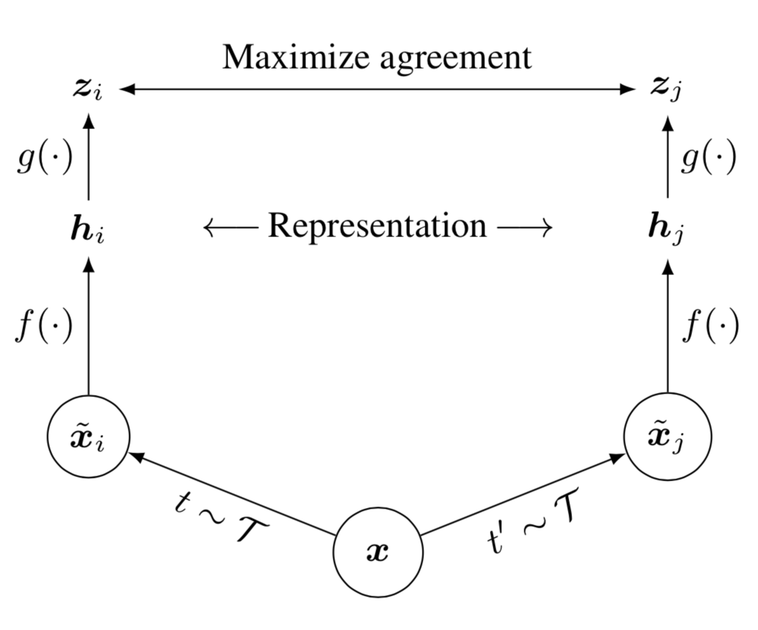
SimCLR [3] employs Contrastive Learning to learn embeddings which can be used for various downstream tasks (supervised-learning tasks using a pre-trained model or component), by the following steps:
1. Randomly sample a minibatch of $N$ samples and each sample $x$ is applied with two different data augmentation operations $t$ and $t'$, resulting in $2N$ augmented samples in total. $\tilde{\mathbf{x}}_i = t(\mathbf{x}),\quad\tilde{\mathbf{x}}_j = t'(\mathbf{x}),\quad t, t' \sim \mathcal{T}$ where $t$ and $t'$ are sampled from the same family of augmentations $\mathcal{T}$, which includes random crop, resize with random flip, color distortions, and Gaussian blur.
2.Given one positive pair$(\tilde{\mathbf{x}}_i, \tilde{\mathbf{x}}_j)$, other $2(N-1)$ data points are treated as negative samples. The representations of these augmented samples are produced by a base encoder $f(.)$, i.e., $\mathbf{h}_i = f(\tilde{\mathbf{x}}_i),\quad \mathbf{h}_j = f(\tilde{\mathbf{x}}_j)$. Moreover, the representation $\mathbf{h}$ is used for downstream tasks.
3. The contrastive learning loss is defined using cosine similarity $\mbox{sim}(.,.)$, which operates on an extra projection layer of the representation $g(.)$ rather than on the representation space $\mathbf{h}$ directly. The importance of using the representation before the nonlinear projection is due to loss of information (which is used for downstream tasks) induced by the contrastive loss. For each pair of $(\mathbf{h}_i, \mathbf{h}_j)$, the loss is defined by the following
$$ \mathbf{z}_i = g(\mathbf{h}_i)$$ $$\mathbf{z}_j = g(\mathbf{h}_j) $$ $$ \mathcal{L}_\text{SimCLR}^{(i,j)} = - \log\exp(\text{sim}(\mathbf{z}_i, \mathbf{z}_j) / \tau) + \log\sum_{k=1}^{2N} \mathbb{1}_{[k \neq i]} \exp(\text{sim}(\mathbf{z}_i, \mathbf{z}_k) / \tau) $$ $$ =- \log\frac{\exp(\text{sim}(\mathbf{z}_i, \mathbf{z}_j) / \tau)}{\sum_{k=1}^{2N} \mathbb{1}_{[k \neq i]} \exp(\text{sim}(\mathbf{z}_i, \mathbf{z}_k) / \tau)} $$where $\tau$ is the temperature parameter, $\mbox{sim}(.,.)$ is the cosine similarity, and $\mathbb{1}_{[k \neq i]}$ is an indicator function: 1 if $k \neq i$ 0 otherwise.
Barlow Twins
Barlow Twins [4] learns to make the cross-correlation matrix between these two groups of output features close to the identity. The goal is to keep the representation vectors of different distorted versions of one sample similar, while minimizing the redundancy between these vectors.
Let $C$ be a cross-correlation matrix computed between outputs from two identical networks along the batch dimension. Each entry $C_{ij}$ in the matrix is the cosine similarity between $z^A_{b,i}$ and $z^B_{b,j}$.
Then the loss of Barlow Twins is defined by the following
$$\mathcal{L}_{BT}=\sum_i(1-C_{ii})^2+\lambda \sum_i\sum_{j\neq i}C_{ij}^2$$.MoCo
Momentum Contrast (MoCo) [5] trains a visual representation encoder by matching an encoded query $q$ to a dictionary of encoded keys $\{k_1,k_2,...\}$ using the InfoNCE contrastive loss. The query representation is $q = f_q(x_q)$ where $f_q$ is an encoder network and $x_q$ is a query sample (likewise, $k = f_k(x_k)$).
Dictionary as a queue: The samples in the dictionary are progressively replaced. The current mini-batch is enqueued to the dictionary, and the oldest mini-batch in the queue is removed. The advantage of MoCo compared to SimCLR is that MoCo decouples the batch size from the number of negatives, but SimCLR requires a large batch size in order to have enough negative samples and suffers performance drops when their batch size is reduced.
Momentum update: Let $\theta_k$ be the parameters of $f_k$ and $\theta_q$ be those of $f_q$, then $\theta_k$ is updated by the following
$$\theta_k \leftarrow m\theta_k+(1-m)\theta_q,$$
where a relatively large momentum (e.g., m = 0.999, the default) works much better than a smaller value (e.g., m = 0.9).

SwAV
Similarly to contrastive approaches, SwAV [6] learns representations by comparing transformations of an image, but unlike contrastive methods, it does not require to compute feature pairwise comparisons. SwAV also does not require a large memory bank or a special momentum network.- Use a “swapped” prediction mechanism to predict the code of a view from the representation of another view. In particular, given two image features $z_t$ and $z_s$ from two different augmentations of the same image, their codes $q_t$ and $q_s$ are computed by matching to a set of $K$ prototypes $\{c_1,\dots, c_K\}$. Then, the loss is defined by $\mathcal{L}(z_t,z_s) = \mathcal{l}(z_t,q_s)+\mathcal{l}(z_s,q_t)$. If these two features capture the same information, it should be possible to predict the code from the other feature.
- They propose multi-crop that uses smaller-sized images to increase the number of views (transformations per image) while not increasing the memory or computational requirements during training, where mapping small parts of a scene to more global views by the “swapped” prediction mechanism significantly boosts the performance.

SSL in multimodal learning
CLIP
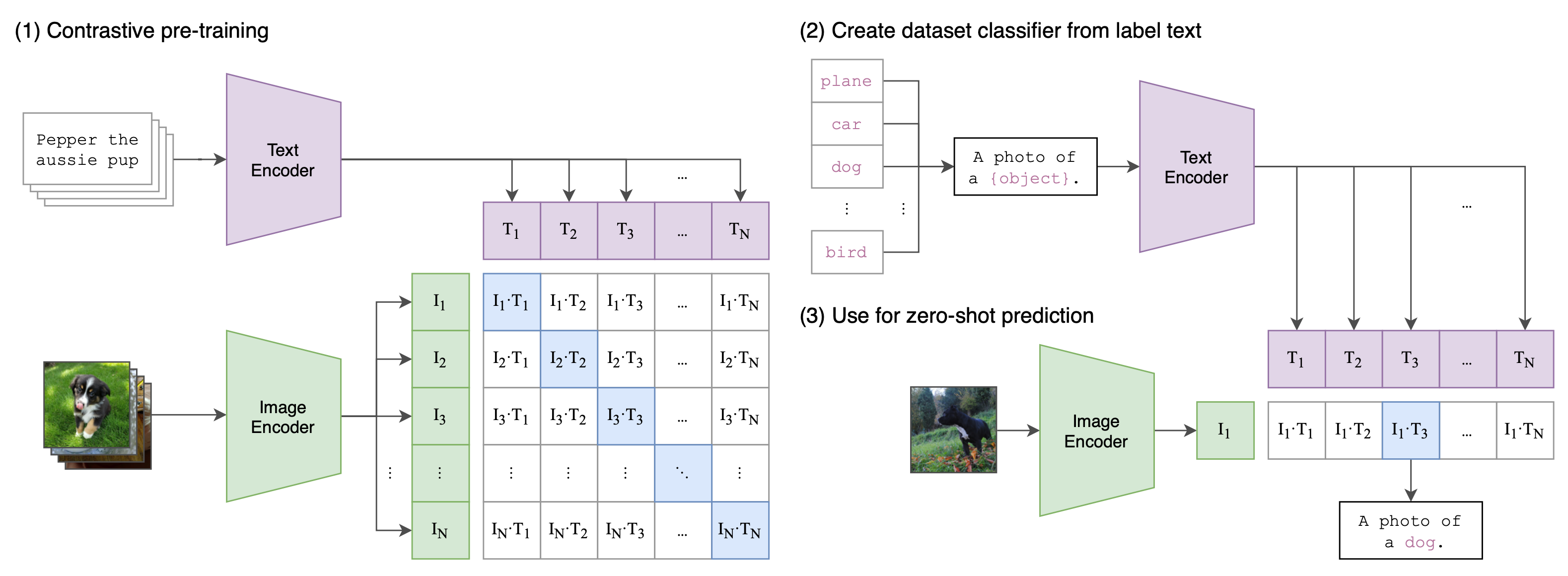
Given a batch of $N$ (image, text) pairs, CLIP [7] computes the dense cosine similarity matrix between all possible (image, text) candidates within this batch. The text and image encoders are jointly trained to maximize the similarity between $N$ correct pairs of (image, text) associations while minimizing the similarity for $N(N-1)$ incorrect pairs via a symmetric cross entropy loss over the dense matrix. It is trained on 400 million (text, image) pairs, collected from the Internet.
MMV
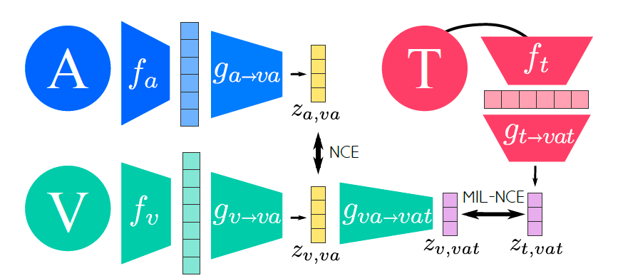
- MultiModal Versatile Networks (MMV) [8] demonstrate how networks trained on large collections of unlabelled video data can be applied on video, video-text, image and audio downstream tasks.
- Multimodal contrastive loss. Concretely, positive training pairs across two modalities are constructed by sampling the two streams from the same location of a video. Conversely, negative training pairs are created by sampling streams from different videos. In particular, minibatch of $N$ video samples is formed, which induces $N$ positive and $N(N-1)$ negative pairs. Given these positive and negative training pairs, similarly, multimodal contrastive loss aims to make the positive pairs similar and negative pairs dissimilar in their corresponding joint embedding, by the following $$\mathcal{L}(x)=\lambda_{va}NCE(x_v,x_a)+\lambda_{vt}MIL-NCE(x_v,x_t),$$ where $\lambda_{mm'}$ corresponds to the weight for the modality pair $m$ and $m'$, $x_v$ denotes the video input, $x_a$ is the audio input, and $x_t$ is the text input. NCE stands for Noise-Contrastive Estimation[9], which is a loss function similar to the contrastive learning loss in SimCLR. Moreover, the MIL-NCE variant is tailored to account for the misalignment between narrations and what is actually happening in the video.


AVLnet [10]
Several differences compared with MMV:- Only consider visual and audio embedding spaces, but the audio is from the same video.
- Using a nonlinear activation layer for attaining feature embeddings.
Datasets
HowTo100M [11]
HowTo100M is a large-scale dataset of narrated videos with an emphasis on instructional videos where content creators teach complex tasks with an explicit intention of explaining the visual content on screen.- 136M video clips with captions sourced from 1.2M Youtube videos (15 years of video).
- 23k activities from domains such as cooking, hand crafting, personal care, gardening or fitness.
- Each video is associated with a narration available as subtitles automatically downloaded from Youtube.