On the Versatility of Transformers

Created by Yuwei Sun
All posts

Key Characteristics of Transformers

• Transformers facilitate modeling of long-term dependencies between input sequence elements by using self-attention mechanisms that allow each element in the sequence to attend to all other elements, enabling the model to capture complex relationships between distant elements.
• Transformers enable efficient parallel processing of sequences on GPUs, compared to RNNs which require sequential processing.
• Transformer models lack inherent inductive biases, which means they do not have any preconceived notions or assumptions about the data they are trained on, and instead rely on learning patterns solely from the input data. This makes them highly flexible and capable of capturing complex relationships in the data, but also means that they require a vast amount of training data to generalize well, and may struggle with low-resource settings or out-of-distribution examples.

Attention Mechanism in Transformers

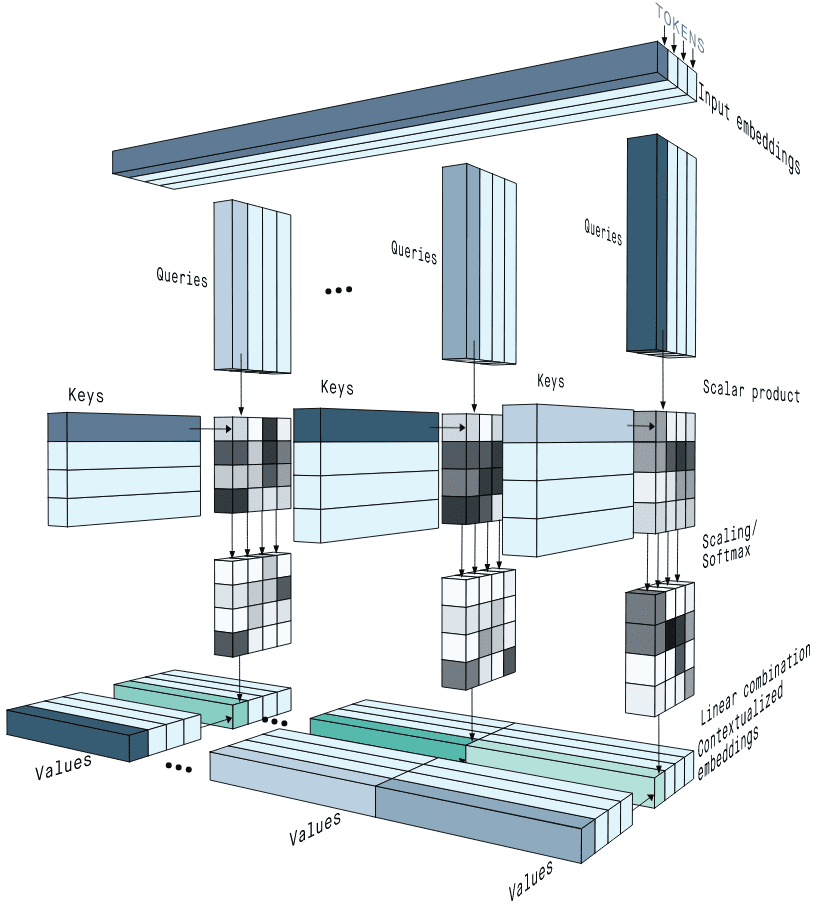
The self-attention mechanism [1] in Transformer models employs multi-head attention in which each head maps a query and a set of key-values pairs to an output (Figure 1). The output in a single head is computed as a weighted sum of values according to the attention score computed by a function of the query with the corresponding key. Let $Q$, $K$, and $V$ be the query, key, and value, respectively. These single-head outputs are then concatenated and projected, resulting in the final values.

$$\mbox{Multi-head}(Q,K,V)=\mbox{Concat}(\mbox{head}^1,\dots,\mbox{head}^H)W^O,$$ $$\mbox{head}^i=\mbox{Attention}(QW^{Q_i},KW^{K_i},VW^{V_i})=\mathbf{A_S}\,\mathbf{V},$$ $$\mathbf{A_S} = \mbox{softmax}(\frac{QW^{Q_i} (KW^{K_i})^T}{\sqrt{d}}),$$

where $W^Q,W^K,W^V$ and $W^O$ are linear transformations for queries, keys, values and outputs. $d$ denotes the dimension of queries and keys in a single head. In self-attention modules, $Q = K = V$.

Transformers in NLP

BERT: Bidirectional Encoder Representations from Transformers [2]

Transfer learning with language models is crucial for language understanding systems, and recent improvements demonstrate that even low-resource tasks can benefit from deep architectures. Bidirectional Encoder Representations from Transformers (BERT) further generalizes these findings to deep bidirectional models.

The model architecture of BERT is based on [1]. The learning framework involves two steps, that is, pre-training and fine-tuning (Figure 2). During pre-training, the model is trained on unlabeled data over different tasks, while for fine-tuning, the model is initialized with the pre-trained parameters and fine-tuned using labeled data from downstream tasks. The input of one token sequence can represent both a single sentence and a pair of sentences (e.g., ⟨ Question, Answer ⟩) separated by a special token ([SEP]). In addition, the first token of every sequence is a special classification token ([CLS]) that outputs token representations for classification tasks.

To pretrain BERT, two unsupervised tasks are included: 1. Masked LM (MLM) masks some percentage of the input tokens at random, and then predict those masked tokens, and 2. Next Sentence Prediction (NSP) is a binarized prediction task that aims to identify whether a sentence B follows a sentence A. In the pre-training examples, 50% of the time B is the actual next sentence that follows A (labeled as IsNext), and 50% of the time it is a random sentence from the corpus (labeled as NotNext).

RoBERTa: Robustly Optimized BERT Pre-training [3]

Robustly Optimized BERT Pre-training (RoBERTa) is a replication study of BERT to measure the impact of key hyperparameters and training data size. Several modifications compared to BERT include: 1. training the model longer, with bigger batches, over more data, 2. remove the Next Sentence Prediction (NSP) optimization, 3. training on longer sequences, and 4. dynamically changing the masking pattern applied to the training data. These modifications result in a better performance in benchmark NLP tasks.

ChatGPT [4]

ChatGPT is trained to follow an instruction in a prompt and provide a detailed response. The framework is based on GPT-3 (Generative Pre-trained Transformer v3) architecture. By further incorporating Reinforcement Learning from Human Feedback (RLHF), ChatGPT is fine-tuned to generate more accurate and relevant responses to specific prompts based on human feedback.

GPT-3 (Generative Pre-trained Transformer v3) [5]

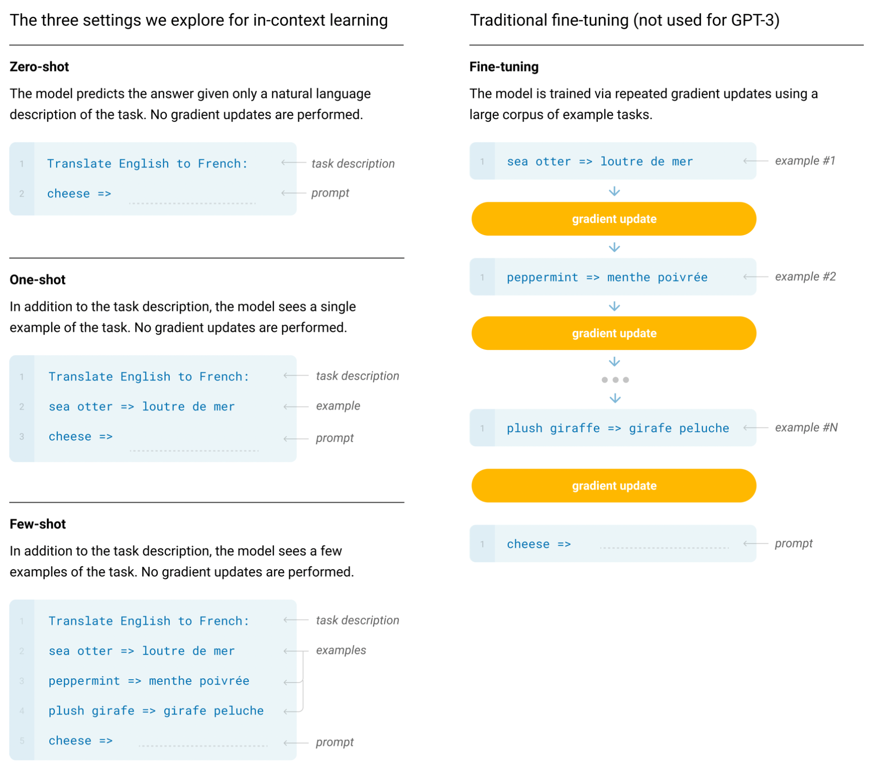
Generative Pre-trained Transformer v3 (GPT-3) is an autoregressive language model with 175 billion parameters. GPT-3 is pre-trained on a large corpus of text data using unsupervised learning. The model is trained using a masked language modeling objective, where a random subset of the input tokens are masked out and the model is tasked with predicting the missing tokens based on the surrounding context. GPT-3 was evaluated under 3 conditions: (a) few-shot learning but no weight updates allowed (typically 10 to 100 demonstrations), (b) one-shot learning, and (c) zero-shot learning with only an instruction in natural language. These conditions are different from the fine-tuning that involves updating the weights of a pre-trained model by training on a supervised dataset specific to the desired task (Figure 3).

RLHF: Reinforcement Learning from Human Feedback [6]

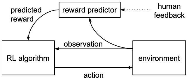
Reinforcement Learning from Human Feedbacks (RLHF) enables human trainers to guide the learning process of an agent by providing feedback on its behavior (Figure 4). In particular, given a policy network $\pi : O → A$ and a reward function that estimates $\hat{r}: O × A → R$, these networks are updated by the following three processes:

• 1. The policy $\pi$ interacts with the environment to produce a set of trajectories $\{\tau_1,...,\tau_i\}$, where $\pi$ is updated by a traditional reinforcement learning algorithm, to maximize the sum of the predicted rewards $r_t = \hat{r}(o_t, a_t)$.
• 2. Select pairs of segments $(\sigma^1, \sigma^2)$ from the trajectories $\{\tau_1,...,\tau_i\}$ produced in step 1, and send them to a human for comparison.
• 3. The parameters of the mapping $\hat{r}$ are optimized via supervised learning to fit the comparisons collected from the human so far.

To optimize $\hat{r}$, the human indicates which segment they prefer, that the two segments are equally good, or that they are unable to compare the two segments, which are recorded in a database $D$ of triples $(\sigma^1, \sigma^2, \mu)$, where $\mu$ is a distribution over {1, 2} indicating which segment the user preferred. If the human selects one segment as preferable, then $\mu$ puts all of its mass on that choice. If the human marks the segments as equally preferable, then $\mu$ is uniform. Finally, if the human marks the segments as incomparable, then the comparison is not included in the database.

$$\hat{P}[\sigma^1 \mathcal{>} \sigma^2] = \frac{\mbox{exp}\sum \hat{r}(o_t^1, a_t^1)}{\mbox{exp}\sum \hat{r}(o_t^1, a_t^1)+\mbox{exp}\sum \hat{r}(o_t^2, a_t^2)},$$

where $\hat{r}$ is minimized with the cross-entropy loss between these predictions and the actual human labels.

$$\mbox{loss}(\hat{r}) = -\underset{(\sigma^1, \sigma^2, \mu) \in D}{\sum} \mu(1) \mbox{log}\hat{P}[\sigma^1 \mathcal{>} \sigma^2] + \mu(2) \mbox{log}\hat{P}[\sigma^2 \mathcal{>} \sigma^1].$$

LoRA (Low-Rank Adaptation) [7]

Low-Rank Adaptation (LoRA) in Transformer models is a fine-tuning approach that greatly reduces the number of trainable parameters for downstream tasks. To achieve this goal, LoRA freezes the pre-trained model weights and injects trainable rank decomposition matrices into each layer of the Transformer architecture (Figure 5). Moreover, in the Transformer architecture, there are weight matrices in both the self-attention module ($W^Q, W^K, W^V, W^O$) and the MLP module. LoRA adopts the rank decomposition to the attention weights and freezes the MLP modules (so they are not trained in downstream tasks) for simplicity and parameter-efficiency.

For a pre-trained weight matrix $W_0 \in \mathbb{R}^{d\times k}$, LoRA constrain its update by representing the latter with a low-rank decomposition $W_0 + \Delta W = W_0 + BA$, where $B \in \mathbb{R}^{d\times r}, A\in \mathbb{R}^{r\times k}$, and the rank $r \ll \mbox{min}(d,k)$. During training, $W_0$ is frozen and does not receive gradient updates, while $A$ and $B$ contain trainable parameters. Then, for $h = W_0x$, the forward pass yields $h = W_0x + \Delta Wx = W_0x + BAx$, which are summed coordinate-wise.

Transformers in Vision

ViT (Vision Transformers) [8]

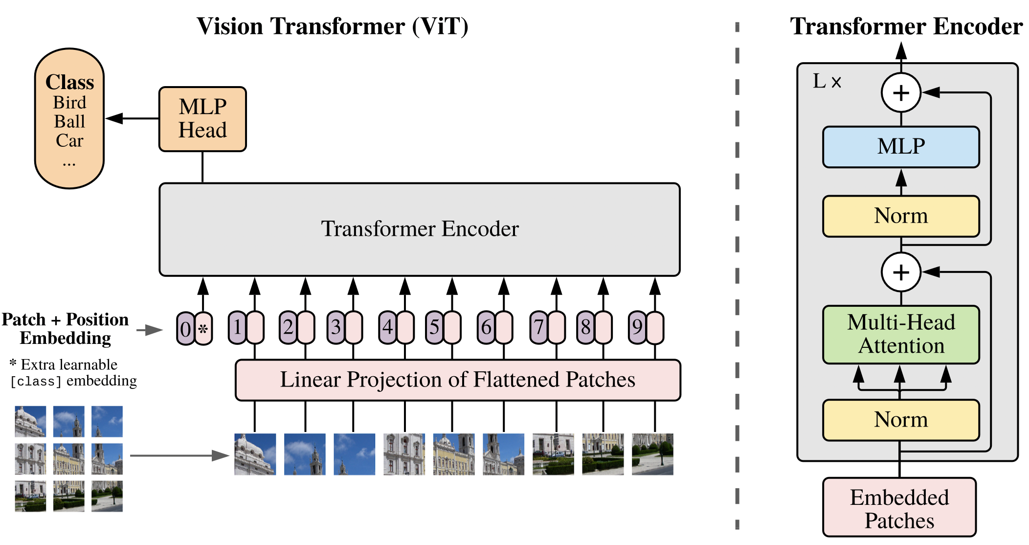
Vision Transformers (ViT) can achieve excellent results on image classification tasks by directly processing sequences of image patches (Figure 6). Let $x\in\mathbb{R}^{H\times W\times C}$ be an image input, where $(H,W)$ is the resolution of the image and $C$ is the number of channels. $x$ is separated into a sequence of 2D patches $x_p\in \mathbb{R}^{N\times (P^2\cdot C)}$ ,where $(P,P)$ is the resolution of each image patch and $N=\frac{HW}{P^2}$ is the number of patches. Similar to Transformers in NLP, these patches are mapped to $D$ dimensions with a trainable linear projection whose output is called the patch embeddings. Learnable 1D position embeddings are added to the patch embeddings to retain positional information. Moreover, a learnable [class] token embedding is prepended to the sequence of embedded patches $(z_0^0 = x_{\mbox{class}})$, whose state at the output of the Transformer encoder, $(z^0_L)$, serves as the image representation for downstream tasks. Both during pre-training and fine-tuning, a classification head is attached to $(z^0_L)$ for a classification task, which is implemented by a MLP with one hidden layer at pre-training time and by a single linear layer at fine-tuning time.

Nevertheless, since ViT lacks the inductive biases inherent to CNNs like translation equivariance and locality, it yields modest accuracies a few percentage points below ResNets of comparable size when trained on mid-sized datasets such as ImageNet without strong regularization.

Swin (Shifted Windows) Transformer [9]

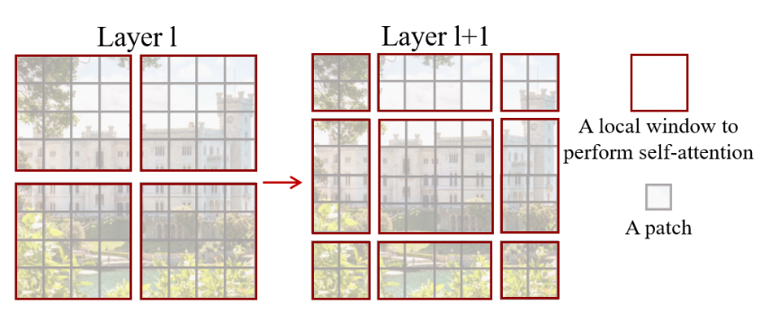
Swin Transformer splits an input RGB image into non-overlapping patches by a patch splitting module (Figure 7). Each patch is treated as a “token” and its feature is set as a concatenation of the raw pixel RGB values. Given an image with a size $W\times H \times C$ and a patch size of $4\times 4$, the Transformer blocks maintain the number of tokens $(\frac{W}{4}\times \frac{H}{4})$. Thrn, different from ViT, the number of tokens is reduced by patch merging layers as the network gets deeper. The first patch merging layer concatenates the features of each group of 2 × 2 neighboring patches, and applies a linear layer on the $4C$-dimensional concatenated features. Furthermore, Swin Transformer blocks based on shifted windows are applied afterwards, where the self-attention is computed within the non-overlapping local windows of the merged patches. The resolution of patches is kept at $(\frac{W}{8}\times \frac{H}{8})$. Such procedure is repeated twice with output resolutions of $(\frac{W}{16}\times \frac{H}{16})$ and $(\frac{W}{32}\times \frac{H}{32})$, respectively. This strategy allows reduced computational complexity.

To learn cross-window connections while maintaining the efficient computation within non-overlapping windows, Swin Transformer employs a shifted window partitioning startegy which alternates between two partitioning configurations in consecutive Swin Transformer blocks (Figure 8). In particualr, the first block uses a regular window partitioning strategy which starts from the top-left pixel, and the 8×8 feature map is evenly partitioned into 2×2 windows of size 4×4. Then, the next block adopts a windowing configuration that is shifted from that of the preceding block, by displacing the windows by ($\frac{M}{2}$, $\frac{M}{2}$) pixels from the regularly partitioned windows.

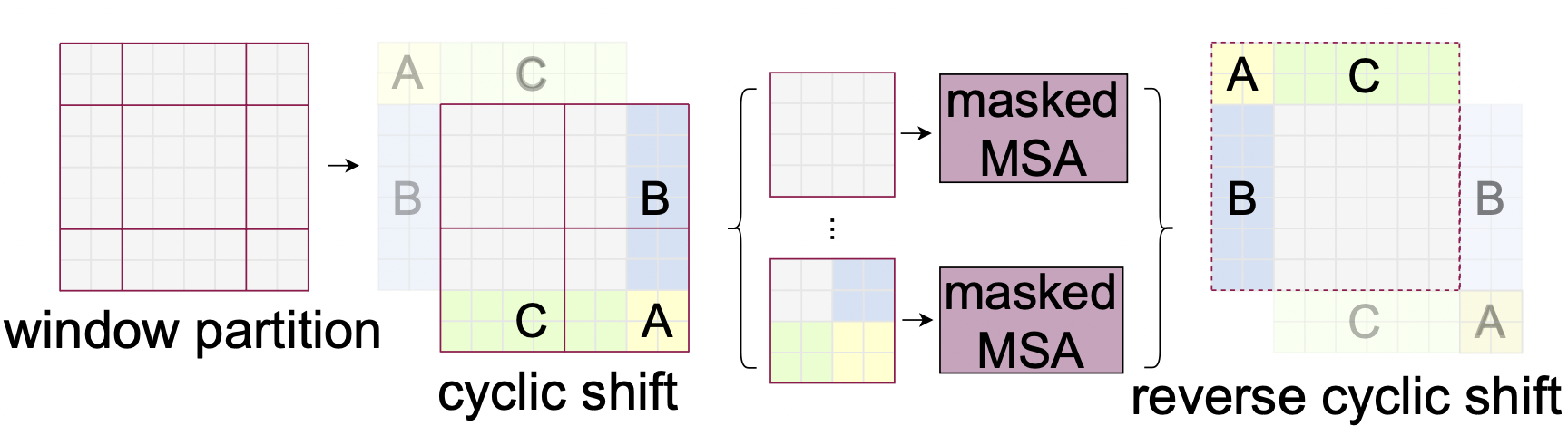
However, an issue with the shifted window partitioning is that it will result in more windows, from $\frac{h}{M}$×$\frac{w}{M}$ to ($\frac{h}{M}$+1)×($\frac{w}{M}$+1), and some of the windows will be smaller than $M × M$. A masking mechanism is employed to limit self-attention computation to within each sub-window, such that the number of batched windows remains the same as that of regular window partitioning (Figure 9).

Transformer in Reinforcement Learning

Decision Transformer [10] introduces a framework that abstracts Reinforcement Learning (RL) as a sequence modeling problem, by modeling the joint distribution of states, actions, and rewards sequences (Figure 10). Decision Transformer employs as the input the trajectory representation $\tau$ of the returns-to-go $\hat{R}_t=\sum_{t^\prime=t}^T r_{t^\prime}$, states $s_t$, and actions $a_t$. $\tau=(\hat{R}_1,s_1,a_1,\hat{R}_2,s_2,a_2,...,\hat{R}_T,s_T,a_T)$. To obtain token embeddings, a linear layer followed by layer normalization is employed. For environments with visual inputs, the state is fed into a convolutional encoder instead of a linear layer. Besides the states, actions, and returns, an embedding for each timestep is learned and added to each token, with one timestep $t$ corresponding to three tokens ($\hat{R}_t,s_t,a_t$).

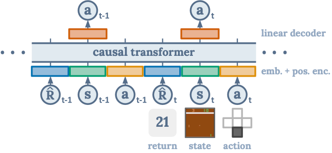
For training, given a dataset of offline trajectories, minibatches of sequence length $K$ are sampled from the dataset. The obtained token embeddings are then fed into a GPT architecture which predicts actions autoregressively using a self-attention mask. The prediction head corresponding to the input token $s_t$ in the GPT architecture, is trained to predict $a_t$, either with cross-entropy loss for discrete actions or mean-squared error for continuous actions. The losses at each timestep in the minibatch are averaged for the model training.