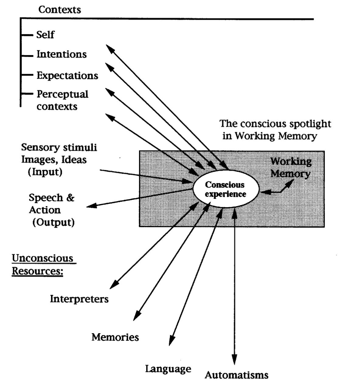
The global workspace theory [1] demonstrated that in the human brain, multiple neural network models cooperate and compete in solving problems via a shared feature space for common knowledge sharing, which is called the global workspace (GW).
Fig.1 - A schematic diagram of GW theory.
GW is closly connected to System 1 and System 2 AI [2]. System 2 cognition is thought to reject, alter, or overcome impressions, intuitions, feelings, and reactive tendencies that are issued by System 1. System 2 can also fully endorse and select from the bottom-up inputs provided by System 1. System 1 cognition translates to all automatic, over-learned processes that may engage relatively local specialized networks. In contrast, System 2 cognition would engage effortful cognitive processes that rely on more distributed processing of collective networks and flexible interactions between these specialized neural systems. Conscious attention selects which module and conscious content is gated through this bottleneck and remains available shortly in working memory [3].
Common Sense is a Collection of Models of the World
Within the global workspace theory, using different kinds of metadata about individual neural networks such as measured performance and learned representations, shows the potential to learn, select, or combine different learning algorithms to efficiently solve a new task. The learned knowledge or representations from different neural network areas are leveraged for reasoning and planning. This research area studies how a meta agent can solve novel tasks by observing and leveraging the world models built by these individual neural networks. Common sense is not just facts but a collection of models of the world.
Learning from Many Replica Neural Networks
The proliferation of AI applications is reshaping the contours of the future knowledge graph of neural networks. Decentralized NNs is the study of knowledge transfer from different individual neural networks trained on separate local tasks to a global model. In a learning system comprising many replica neural networks with similar architecture and functions, the goal is to learn a global model that can generalize to unseen tasks without large-scale training [4]. Sometimes, we call the different replica models the local models. In particular, two piratical problems in Decentralized NNs are being intensively studied, i.e., learning with non-independent and identically distributed (non-iid) data and multi-domain data.
Notably, non-iid refers to data samples across local models are not from the same distribution, which hinders the knowledge transfer between local models. To tackle the non-iid problem, we proposed the Segmented-Federated Learning (Segmented-FL) [5] that employs periodic local model performance evaluation and learning group segmentation that brings neural networks training over similar data distributions together. Then, for each group, Segmented-FL trains a different global model by transferring knowledge from the local models in the group. The global model can only passively observe the local model performance without access to the local data. Segmented-FL can achieve better performance in tackling non-iid data compared to the traditional federated learning [6].
On the other hand, multi-domain refers to data samples across local models are from different domains with domain-specific features. For example, an autonomous vehicle learns to drive in a new city might leverage the driving data of other cities learned by different vehicles. Since different cities have different street views and weather conditions, it would be difficult to directly learn a new model based on the knowledge of the models trained on multi-domain data. This problem is closely related to multi-source domain adaptation, which studies the distribution shift in features inherent to specific domains that brings in negative transfer degrading a model's generality to unseen tasks. A detailed blog on Domain Shift and Transfer Learning.
Building the Hierarchy of Neural Networks
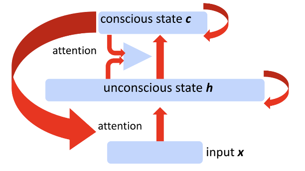
Fig.2 - Concious and unconcious states.
Hierarchical neural networks consist of multiple neural networks concreted in a form of an acyclic graph. An early theory of the global workspace theory (GWT) [1] refers to multiple neural network models cooperating and competing in solving problems via a shared feature space for common knowledge sharing. Built upon the GWT, the conscious prior theory [7] demonstrated the sparse factor graphs in space of high-level semantic variables and simple mapping between high-level semantic variables. The hierarchy of neural networks usually comprises two learning frameworks, i.e, fast learning and slow learning [2]. The fast learning framework comprises different individual modules while the slow learning framework is more like an attention mechanism for long-term planning.
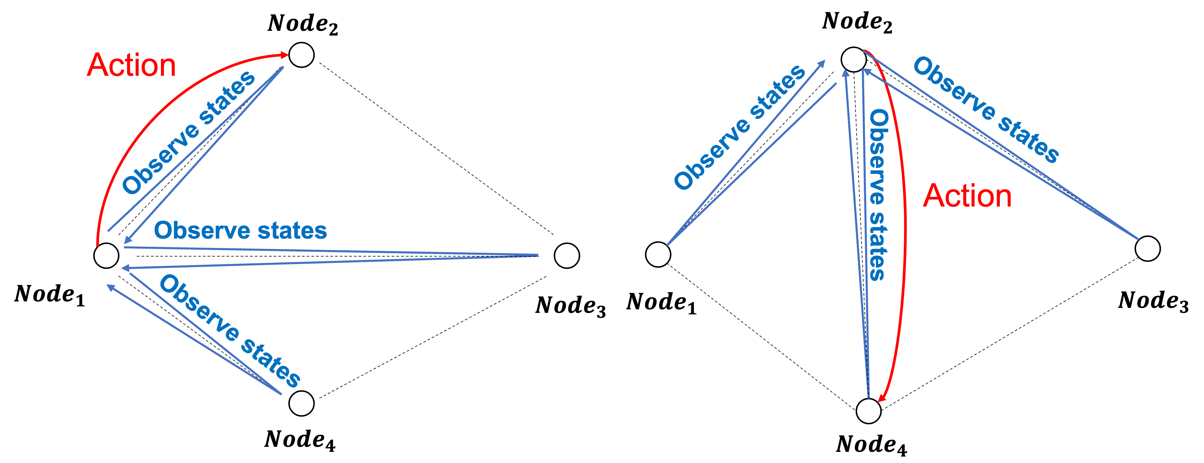
Fig.3 - Homogeneous learning.
In particular, Homogeneous learning [8] introduced a self-attention mechanism where a local model is selected as the meta for each training round and leverages reinforcement learning to recursively update a globally shared learning policy. The meta observes the states of local models and its surrounding environment, computing the expected rewards for taking different actions based on the observation. As mentioned in [9], with a model of external reality and an agent's possible actions, it can try out various alternatives and conclude which is the best action using the knowledge of past events. The goal is to learn an optimized learning policy such that the Decentralized NNs systems can quickly solve a problem by planning and leveraging different local models' knowledge more efficiently. The results showed that the learning of a learning policy greatly reduced the total training time for a given classification task by 50.8%.
Leveraging Different Modality Experts
Information in the real world usually comes in different modalities. The degeneracy[10] in neural structure refers to any single function can be carried out by more than one configuration of neural signals and different neural clusters participate in several different functions. Intelligence systems build models of the world with different modalities where spatial concepts are generated via different modality models. The cross-modal learning in multimodal models such as the Visual Question Answering (VQA) problem can be tackled with approaches such as self-supervised learning [11]. For instance, UniCon [12] leverages the contrastive learning of different model components to align the modality representations encouraging the similarity of the relevant component outputs while discouraging the irrelevant outputs. Such that the learning framework learns better-refined cross-modal representations for unseen VQA tasks based on the knowledge learned from different VQA tasks of local models. A detailed blog on Self-Supervised Learning and Multimodal Learning.
Related Work
Attention
The self-attention module in models like Transformer [13] employs the multi-head attention mechanism in which each head maps a query and a set of key-values pairs to an output. The output in a single head is computed as a weighted sum of values according to the attention score computed by a function of the query with the corresponding key. These single-head outputs are then concatenated and again projected, resulting in the final values:
$$\mbox{Multi-head}(Q,K,V)=\mbox{Concat}(\mbox{head}^1,\dots,\mbox{head}^H)W^O,$$
$$\mbox{head}^i=\mbox{Attention}(QW^{Q_i},KW^{K_i},VW^{V_i}),$$
$$\mathbf{A_S} = \mbox{Attention}(Q,K,V)=\mbox{softmax}(\frac{QK^T}{\sqrt{d}}),$$
$$\mathbf{A_R}=\mathbf{A_S}\,\mathbf{V},$$
where $W^Q,W^K,W^V$ and $W^O$ are linear transformations for queries, keys, values and outputs. $\tilde{Q}= QW^{Q_i}$, $\tilde{K} = KW^{K_i}$, and $\tilde{V} = VW^{V_i}$. $d$ denotes the dimension of queries and keys in a single head. In self-attention modules, $Q = K = V$.
Together, modularity (Global Workspace Theory) and attention direct information flow, which leads to reliable performance improvements in perceptual and language tasks, and in particular improves robustness to distractions and noisy data.
Learning to Combine Top-Down and Bottom-Up Signals in Recurrent Neural Networks with Attention over Modules [14]
Fig.4 - Illustration of Recurrent Independent Mechanisms (RIMs).
This work extended Recurrent independent mechanisms (RIMs) [15] to a multilayered bidirectional architecture, which they refer to as BRIMs. Each layer is a modified version of the RIMs architecture.
Similar to RIMs, the hidden state $h^l_t$ on each layer $l$ and time $t$ is decomposed into separate
modules, which can be represented as $\{((h^l_{t,k})_{k=1}^{n_l}, S_t^l)\}$ where $n_l$ denotes the number of modules in layer $l$ and $S_t^l$ is the set of modules that are active at time $t$ in layer $l$. $|S_t^l| = m_l$, where $m_l$ is the number of modules active in layer $l$ at any time. Each layer can potentially have different number of modules active. Typically, setting $m_l$ to be roughly half the value of $n_l$ works well.
Fig.5 - Overall layout of the Bidirectional Recurrent Independent Mechanisms (BRIMs) model. Information is passed forward in time using recurrent connections and information passed between layers using attention. Modules attend to both the lower layer on the current time step as well as the higher layer on the previous time step, along with Null, which refers to a vector of zeros.
Communication Between Layers and Sparse Activation
Build multi-layer dependency by considering queries $\bar{\mathbf{Q}}= Q_{lay}(h^l_{t−1})$ from modules in layer $l$ and keys $\bar{\mathbf{K}}= K_{lay}(\emptyset, h^{l-1}_{t}, h^{l+1}_{t-1})$ and values $\bar{\mathbf{V}}= V_{lay}(\emptyset, h^{l-1}_{t}, h^{l+1}_{t-1})$ from all the modules in the lower and higher layers.
Based on the attention score $\bar{A}_S^l$, the set $S_t^l$ is constructed which comprises modules for which Null information is least relevant depending on the choice of active module number. Every activated module gets its own separate version of input which is obtained through the attention output $\bar{A}_R^l$. Concretely, for each activated module, this can be represented as:
$$\bar{h}^l_{t,k} =F_k^l(\bar{A}_{R_k}^l,h^l_{t−1,k})\,\,k\in S_t^l,$$
where $F_k^l$ denotes the recurrent update procedure. Note that each module has its own separate parameters. Aside from being module-specific, the internal operation of the recurrent update such as LSTM and GRU remains unchanged.
Communication Within Layers
Perform communication between the different modules within each layer. $\hat{\mathbf{Q}}=Q_{com}(\hat{h}^l_t)$ from active modules.
$\hat{\mathbf{K}}=K_{com}(\hat{h}^l_t)$ and $\hat{\mathbf{V}}=V_{com}(\hat{h}^l_t)$ from all the modules to get the final update to the module state through residual attention $\hat{A}_R^l$ addition. $h^l_{t,k}=\bar{h}^l_{t,k}+\hat{A}_R^l \,\,k\in S^l_t$. $h^l_{t,k}=h^l_{t-1,k}\,\,k\notin S^l_t$.
Coordination Among Neural Modules Through a Shared Global Workspace [16]
They argue that more flexibility and generalization emerge through an architecture of specialists if their training encourages them to communicate effectively with one another via the bottleneck of a shared workspace.
Writing Information in the shared workspace.
Let matrix $\mathbf{R}$ represent the combined state of all the specialists.The query is a function of the state of the current workspace memory content, represented by matrix $\mathbf{M} = [m_1 ; . . . m_j ; . . . m_{n_m}]$ where $n_m$ is the number of memory slots, i.e $\tilde{\mathbf{Q}}=\mathbf{M}\,\tilde{\mathbf{W}^q}$. Keys and values are a function of the information from the specialists i.e., a function of $\mathbf{R}$. The memory is updated by: $\mathbf{M} ← \mbox{softmax}(\frac{\tilde{\mathbf{Q}}(\mathbf{R}\tilde{\mathbf{W}}^e)^T}{\sqrt{d_e}})\mathbf{R}\tilde{\mathbf{W}}^v.$ Selection of the set of specialists $\mathcal{F}_t$with a top-$k$ softmax is a hybrid between hard and soft selection.
Broadcast of information from the shared workspace.
Each specialist then updates its state using the information broadcast from the shared workspace.
All the specialists create queries $\hat{q}_k = h^k_t\hat{\mathbf{W}}^q$, which are matched with the keys $\hat{k}_j=(m_j\hat{\mathbf{W}}^e)^T\,\,\forall k \in \{1,...,n_s\}, j \in \{1,...,n_m\}$ from the updated memory slots, where $n_s$ is the number of modules and $n_m$ is number of memory slots. The memory slot values generated by each slot of the shared workspace and the attention weights are then used to update the state of all the specialists: $h_t^k \leftarrow h_t^k + \sum_j \mbox{softmax}(\frac{\hat{q}_k\hat{k}_j}{\sqrt{d_e}})m_j\hat{\mathbf{W}}^v \,\,\forall k\in \{1,...,n_s\}$.
After receiving the broadcast information from the workspace, each specialist update their state by applying some dynamics function i.e., LSTM or GRU units. This yields the new value $h^k_{t+1}$ for the $k$-th specialist.
Discrete valued neural communication with global workspace theory [17]
Subsymbolic architectures, like neural networks, utilize continuous representations and statistical computation. On the other hand, symbolic architectures, like production systems and traditional expert systems, use discrete, structured representations and logical computation.
This work introduced a discrete latent space vector $e\in \mathbb{R}^{L\times(m/G)}$ where $L$ is the size of the discrete latent space (i.e., an $L$-way categorical variable), and $m$ is the dimension of each latent embedding vector $e_j$. Here, $L$ and $m$ are both hyperparameters. In addition, by dividing each target vector into $G$ segments or discretization heads, they separately quantize each head and concatenate the results.
In particular, a vector $h$ is divided into $G$ segments $s_1, s_2, . . . , s_G$ with $h = \mbox{CONCAT}(s_1, s_2, . . . , s_G)$, where each segment $s_i \in \mathbb{R}^{m/G}$ with $\frac{m}{G}\in \mathbb{N}+$. Second, each segment $s_i$ is discretized separately:
$$e_{o_i} = DIS(s_i),$$
where $o_i = \underset{j \in {1,...,L}}{\mbox{arg min}}||s_i - e_j||$.
Finally, concatenate the discretized results to obtain the final discretized vector $Z$ as $Z = \mbox{CONCAT}(DIS(s_1), DIS(s_2), ..., DIS(s_G))$.
$e$ is shared across all communication vectors and heads, and is trained together with other parts of the model.
The overall loss for model training is:
$$\mathcal{L} = \mathcal{L}_{task}+\frac{1}{G}(\sum_i^G||sg(s_i)-e_{o_i}||_2^2+\beta\sum_i^G||s_i-sg(e_{o_i})||_2^2 ),$$
where $sg$ refers to a stop-gradient operation that blocks gradients from flowing into its argument.
In recurrent independent mechanisms (RIMs), outputs from different modules are communicated to each other via soft attention mechanism. In the original RIMs method, $\tilde{z}_i^{t+1}=RNN(z_i^t,x^t)$ for active modules, and $\tilde{z}_{i'}^{t+1}=z_{i'}^t$ for inactive modules where $t$ is the time step, $i$ is index of the module, and $x^t$ is the input at time step $t$. Then, the dot product query-key soft attention is used to communication output from all modules $i \in \{1, . . . , M\}$ such that $h_i^{t+1} = \mbox{SOFTATTENTION}(\tilde{z}_1^{t+1},\tilde{z}_2^{t+1},\dots,\tilde{z}_M^{t+1})$.
Then, $z_i^{t+1}=\tilde{z}_i^{t+1}+h_i^{t+1}$.
The discretization process of discrete valued neural communication (DVNC) is applied to the output of the soft attention:
$$z_i^{t+1}=\tilde{z}_i^{t+1}+DIS(h_i^{t+1},L,G).$$
[1] Baars, B. J. 1988. A Cognitive Theory of Consciousness. Cambridge University Press.
[2] Kahneman, D. 2011. Thinking, Fast and Slow. In New York: Farrar, Straus and Giroux.
[3] 2021. How does hemispheric specialization contribute to human-defining cognition? Neuron, 109(13): 2075–2090.
[4] Sun, Y.; Ochiai, H.; and Esaki, H. 2021. Decentralized Deep Learning for Multi-Access Edge Computing: A Survey on Communication Efficiency and Trustworthiness. In IEEE Transactions on Artificial Intelligence.
[5] Sun, Y.; Ochiai, H.; and Esaki, H. 2020. Intrusion Detection with Segmented Federated Learning for Large-Scale Multiple LANs. In IJCNN.
[6] McMahan, B.; Moore, E.; Ramage, D.; and et al. 2017. Communication-Efficient Learning of Deep Networks from Decentralized Data. In AISTATS.
[7] Bengio, Y. 2017. The Consciousness Prior. In arXiv. Craik, K. 1967. The Nature of Explanation. In CUP Archive.
[8] Sun, Y.; and Ochiai, H. 2022. Homogeneous Learning: Self-Attention Decentralized Deep Learning. In IEEE Access, volume 10, 7695–7703.
[9] Craik, K. 1967. The Nature of Explanation. In CUP Archive.
[10] Linda B. Smith and Michael Gasser. The development of embodied cognition: Six lessons from babies. 2005.
[11] Alec Radford, Jong Wook Kim, Chris Hallacy, and et al.. Learning transferable visual models from natural language supervision. 2021.
[12] Sun, Y.; and Ochiai, H. 2022. UniCon: Unidirectional Split Learning with Contrastive Loss for Visual Question Answering. In arXiv preprint.
[13] Ashish Vaswani, Noam Shazeer, Niki Parmar, and et al. Attention is all you need. In NeurIPS, 2017
[14] Sarthak Mittal, Alex Lamb, Anirudh Goyal, et al. Learning to combine top-down and bottom-up signals in recurrent neural networks with attention over modules. ICML 2020.
[15] Anirudh Goyal, Alex Lamb, Jordan Hoffmann, et al. Recurrent independent mechanisms. ICLR 2021.
[16] Anirudh Goyal, Aniket Rajiv Didolkar, Alex Lamb, et al. Coordination among neural modules through a shared global workspace. ICLR 2022.
[17] Dianbo Liu, Alex Lamb, Kenji Kawaguchi, et al. Discrete-valued neural communication. NeurIPS 2021.